A general wall boundary condition (HFI interpretation)

Hard wall

Condition to u' normal

The wall boundary condition is implemented entirely following the paper of Tam Tam & Dong (1994). This implementation is kept very generalised according to the concept of Tam. The condition that the normal velocity at the wall has to be zero

$\underline u'\cdot\underline n_w=\underline 0$

must be fulfilled under any PDE used, even with modified governing equations e. g. in a sponge layer.

Construction of the normal velocity

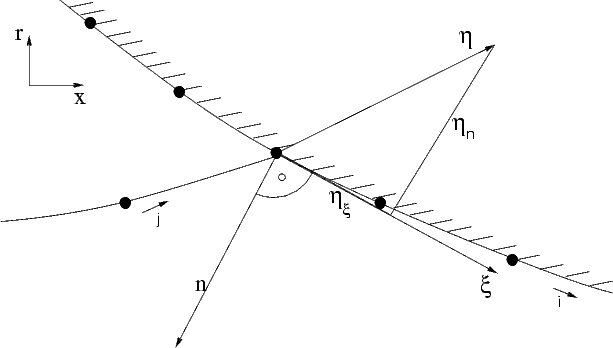
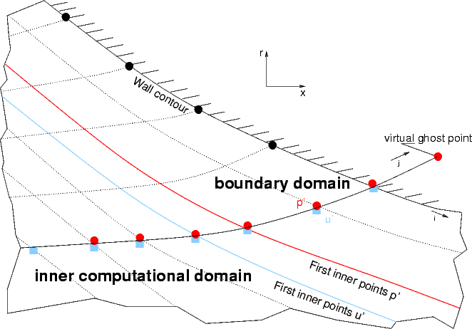
The construction of the wall-normal vector from the body-fitted grid along the wall is shown below.

The ghost point pressure is the key

The consequence for the DRP is the need of an additional degree of freedom to fit this condition. However, the ghost point p'_g does not need to be stored, it is computed on-the-fly from the error made with respect to the u condition using the full PDE. Based on this, the result for the near-wall grid lines is corrected. The steps can be written as follows:

• Backward stencil with PDE in matrix-vector form, this results error due to last ghost pressure
• Update the ghost point p'_g using the backward stencil reversed
• Backward stencil with PDE in matrix-vector form again with only the correction value of p'_g

Implementation details

The area where the values have to be corrected is labeled above as the boundary region. These 3 grid layers before the wall (including the points on the blue line) have to be updated after correction of the ghost point. The concept makes use of the PDE in Matrix-Vector form as it is implemented , so there is no duplicated code. Furthermore, the approach is applicable to any kind of PDE implemented in the code.

Soft wall

Why soft walls?

The soft wall boundary condition is particularly interesting for practical applications, as aero engines usually employ "liners" in the nacelle as a measure to reduce the radiated noise. The time domain description offers the possibility to calculate many frequencies at once, however a model for the frequency dependent complex wall impedance Z_w is needed. Initially, the model of Tam & Auriault (1996) has been implemented to address this issue, and is based on a mechanical analogy model.

Problems with impedance boundary conditions

The technical details are very similar to the hard wall described above, except for the fact that the normal velocity is now given by the complex wall impedance. There are numerous as-yet unresolved problems concerning the soft wall:

• The well-agreed frequency domain boundary condition of Myers (1980) supports unstable solutions when transferred directly to the time domain.
• The use of particle displacement versus the particle velocity is still in discussion.
• The resistance R may vary with frequency, which is not included in the simple mechanical model of Tam & Auriault (1996).
• The causality must be monitored, which is impossible in the time domain.
• The liner may start or end with an abrupt change of the boundary condition applied, and this will excite many modes.

Future work

There are certain specific applications for which this condition leads to a non-valid result, therefore further development in this area is needed. This work is carried out in cooperation with Professor Mei Zhuang (Michigan State University) and Professor Xiaodong Li (Bejing University of Aeronautics and Astronautics)with support of the DAAD.