Various models for sound and perturbations

In this section, various model eqautions and their advantages are discussed. This involves a minimal amount of symbolic formulas, and it may therefore be preferrable to skip this section for first reading.

Model assumptions and consequences

The standard models for aeroacoustics are all based on the linearized Euler equations (LEE). These neglect the influence of friction effects for the propagation of perturbations. Based on this, further model assumptions lead to a variety of different available models.

In the 3D axisymmetric case these are:

• Non-swirling axisymmetric flow (Li et al., 2002; Li et al., 2004) - allows mode decomposition and decoupling of the complex amplitudes
• Axisymmetric swirl flow (Schemel, 2003; Schemel et al., 2004a)
• Acoustic-only (isentropic, non-rotating) propagation (Morgenweck et al., 2004)
• Isentropic assumption for the perturbation (Li et al., 2002; Li et al., 2004) - e. g. for an inlet
• General non-isentropic flow (Schemel et al., 2004b; Schemel, 2003; Schemel et al., 2004a) - e. g. in a combustion chamber

The fully 3D simulation allows:

• Acoustic-only (isentropic, non-rotating) propagation
• Isentropic assumption for the perturbation - e. g. for an inlet (Li et al., 2003)
• General non-isentropic flow - e. g. in a combustion chamber

All of the cases can be combined, and each of the models has its ideal applications. The use of CAA for the non-swirling mean flow in an axisymmetric duct is documented in some recent publications.

The linearized Euler equations (LEE)

Conservation of mass:

$\frac{D \varrho'}{D t} + \bar{\varrho} \underline {\nabla}\cdot \underline... ...bla} \bar{\varrho}+ \varrho' \underline {\nabla}\cdot \underline {\bar U}}= 0$

Conservation of momentum:

$\frac{D \underline {u'} }{D t} + \frac{1}{\bar{\varrho}} \underline {\nabl... ...ine {\bar U} + \underline {u'}\cdot\underline {\nabla} \underline {\bar U}}= 0$

Conservation of energy written as pressure equation

Linearized from the pressure fluctuation:

$\frac{D p'}{D t} + \gamma \bar P \underline {\nabla}\cdot \underline {u... ...rac{p'}{\bar P} \underline {\bar U}\biggr)\cdot\underline {\nabla} \bar P}= 0$

Linearized from the entropy fluctuation:

$\frac{D p'}{D t} + \gamma \bar P \underline {\nabla}\cdot \underline {u... ...\nabla} \bar P + \gamma p' \underline {\nabla}\cdot \underline {\bar U}}= 0$

Matrix-vector-form:

$\frac{\partial \underline q}{\partial t} = - \underline A \cdot \frac{\... ... \cdot \underline q \textcolor{blue}{- \underline D \cdot \underline q}$

Decoupled modes of perturbation in the LEE

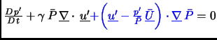
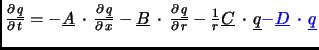
The equations given above describe the propagation of acoustic, vortical and entropic perturbations. These basic perturbations are decoupled in a homogenous flow field. The acoustic perturbation will propagate at the speed of sound relative to the medium, while vorticity and entropy modes are convected. Usually separated length scales for the different modes are found. Please refer to for different models allowing only acoustic waves or vorticity and acoustic modes.

The perturbation modes become coupled in inhomogeneous flow!

The blue terms denote the influence of the spatially-varying mean flow. Such variation couples all modes of fluctuation in the flow field, so that additional source terms arise as the initial perturbation passes an inhomogeneous flow field.

Axisymmetric approach

The Fourier decomposition for 3D axisymmetric CAA is done by replacing all φ derivatives with the im terms from the harmonic approach. The Fourier elements are orthogonal, so that the infinite sum can be decoupled. Far downstream of the sound source this enables observation of the cut-on modes, which are excited on high levels. This kind of noise is referred to as the tonal component of aero engine noise.

A commonly used set of model equations in CAA are the Acoustic Perturbation Equations (APE) (Ewert & Schröder, 2003)

APE differ from the LEE in two ways:

• Only acoustic propagation is modelled
• The source term is given by so-called source filtering in the whole domain.

Therefore in APE approaches, the source and propagation zones may overlap. Contrastingly, in the LEE the interaction of mean-flow and hydrodynamic modes is correctly reproduced at the cost of the increased grid density requirement of the hydrodynamic modes. It is planned to implement the source handling of APE and combine it with acoustic-propagation-only modelling.