Discretization

Spatial discretization

Finite difference approach

The continuous governing equations described in the section above are discretized in space using finite differences. In this approach the derivative is approximated at each grid point by summing the values of neighbouring grid points multiplied by a set of coefficients. It has the general form

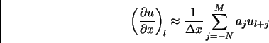$$\left( \frac{\partial u}{\partial x} \right)_l \approx \frac{1}{\Delta x} \sum^M_{j=-N} a_j u_{l+j}$$ (1)

The set a_j is usually called a stencil. The number of points involved in the summation limits the maximal order of accuracy of the approximation.

Dispersion and dissipation error

In acoustical simulations the dispersion error (phase error) and dissipation error (amplitude error) play an important role. Acoustical perturbations can be assumed as physically non-dissipative and nondispersive, propagating with the speed of sound relative to the flow. To ensure accurate reproduction of the amplitude and the phase (propagation speed), high order finite difference schemes are used. Using Fourier analysis, it can be shown that the standard schemes derived for maximal error convergence by the Taylor series expansion have a relatively high dispersion and dissipation at high frequencies, and are suboptimal for the computation of wave propagation. In many publications it has been proved that relaxing the maximal error convergence constraint to the benefit of a wider usable scheme frequency range can increase the overall efficiency, by allowing grids with lower resolution. A widely-used optimized method is the 4th order seven-point central DRP (Dispersion Relation Preserving) scheme of Tam & Webb (1993). This scheme is implemented in the CAA25D code of the HFI.

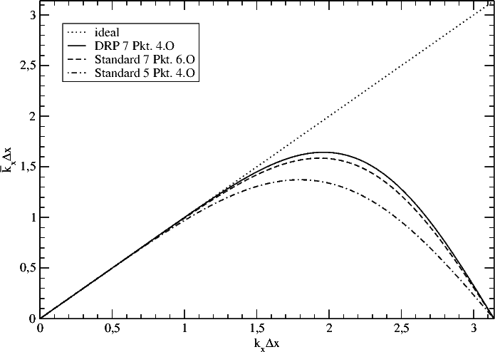
In the diagram below, the dispersion (expressed as the reproduction of the wave number k normalized with the step size of the grid Δ x) is shown for optimized and standard coefficient schemes. The physical wavenumber (abscissa) is plotted vs. the numerical wavenumber (ordinate) approximated by the finite difference scheme.

The dotted line shows the ideal case. It can be observed that the solid line corresponding to the DRP scheme is closer to the ideal line in a much wider frequency range then the dashed line representing the standard scheme. Both schemes have the same computational effort, due to the same number of points in the stencil. For physical wavenumbers where the curve lies below the ideal line, the propagation speed is underestimated and vice-versa. The dissipation diagram is not shown, because a central scheme inherently has no dissipation.

Temporal discretization

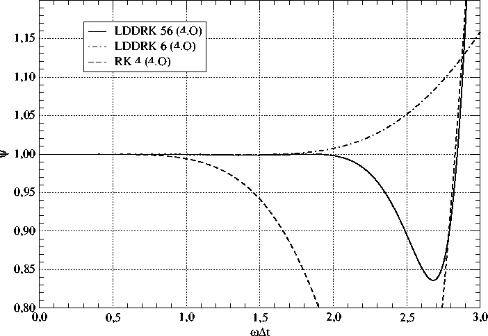
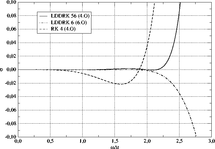
The temporal discretization is achieved using the optimised Runge-Kutta method. This method was introduced by Hu et al. (1996) and is called the Low Dispersion and Dissipation Runge-Kutta (LDDRK) method. In the CAA25D code, the alternating 5/6-step version known as LDDRK56 was implemented. This method invokes an optimized five and six stage scheme of fourth order accuracy alternately with each time step. Both schemes were optimized in combination.

In the diagrams above, the amplitude (upper) and phase (lower) errors compared with the standard RK-method are shown.

Overall efficiency

The time advancing algorithm is implemented in the memory efficient 2-N-storage form described by (Stanescu & Habashi, 1998) and (Williamson, 1980). In this form only two values per degree of freedom must be stored (that is 2 times the number of variables times grid points). This form also simplifies the implementation.