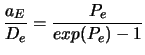
Zur Verdeutlichung des Zusammenhangs zwischen ES und HS erfolgt das
Auftragen von ![]() bzw. seiner dimensionslosen Form
bzw. seiner dimensionslosen Form
![]() als Funktion der Peclet-Zahl
als Funktion der Peclet-Zahl ![]() . Aus (5.26) folgt
. Aus (5.26) folgt
Dieser Verlauf ist im Abbildung 25 dargestellt.
Für positives ![]() ist der Gitterpunkt
ist der Gitterpunkt ![]() der
stromab-Nachbar und sein Einfluß verschwindet mit zunehmendem
der
stromab-Nachbar und sein Einfluß verschwindet mit zunehmendem
![]() . Für negatives
. Für negatives ![]() ist
ist ![]() der stromauf-Nachbar und hat
großen Einfluß.
der stromauf-Nachbar und hat
großen Einfluß.
Einige Eigenschaften des exakten Verlaufs (durchgezogene Linie) sind:
Diese drei Grenzfälle sind ebenfalls im Bild dargestellt
(gestrichelt). Sie formen eine Einhüllende und stellen eine
vernünftige Approximation der exakten Kurve dar. Das Hybrid-Schema
besteht aus diesen drei Geraden, so daß sich ergibt:
oder in Kompaktform:
Signifikanz des HS:
Es ist identisch mit dem CDS für
![]() , und außerhalb
reduziert es sich auf das UDS mit Diffusion
, und außerhalb
reduziert es sich auf das UDS mit Diffusion ![]() .
.
Die Konvektions-Diffusions-Diskretisierungsgleichung für das HS ist also
mit
Diese Formulierung gilt für jede beliebige Lage der
Kontrollvolumen-Wände.
![\includegraphics*[width=11cm, angle=0]{Abb/fvm5_3.eps}](img520.png)
![$\displaystyle a_E = D_e \, [\![ -P_e,\ 1 - {P_e \over 2},\ 0]\!]$](img532.png) bzw.
bzw.![$\displaystyle \qquad a_E = [\![ -F_e,\ D_e - {F_e \over 2},\ 0]\!]$](img533.png)
![$\displaystyle [\![-F_e,\ D_e - {F_e \over 2},\ 0]\!]$](img536.png)
![$\displaystyle [\![+F_w,\ D_w + {F_w \over 2},\ 0]\!]$](img537.png)