Aeroacoustics

Acoustic analogy

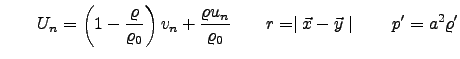
Based on the work of Lighthill and Ffowcs-Williams, the unsteady pressure and velocity fluctuations in the flow field constitute the sources of an inhomogeneous wave equation governing the noise propagation problem. These fluctuating values are obtained by CFD. The equation used for computing the acoustic far-field at different observer positions based on Farassat formulation 1A for penetrable surfaces reads as follows:

$$4 \pi p'(\vec x,t) = \int \limits_{S} \left[\frac {\varrho_{0} (\dot U_{n}+ U_{\dot n}... ...mits_{S} \left[\frac {\varrho_{0} U_{n}K}{r^{2} (1-M_{r})^{3}} \right]_{ret} dS$$

$$+ {1 \over a}\int \limits_{S} \left[\frac {\dot L_{r}}{r (1-M_{r})^... ...r a}\int \limits_{S} \left[\frac {L_{r}K}{r^{2} (1-M_{r})^{3}} \right]_{ret} dS$$

with

$$K = r \dot M_{r}+a M_{r}-a M^{2} \qquad M_{r} = {v_{r} \over a} \qqua... ... = \frac{(x-y)_{i}}{r} L_{i} \qquad L_{i} = \varrho u_{i}(u_{n}-v_{n}) + P_{in}$$

$$P_{in} = (p-p_{0}) n_{i} \qquad \mid \mbox{$\tau_{ij}$\ neglected} \qquad U_{n} = \left(1-{\varrho \over \varrho_{0}}\right)v_{n} +{... ...er \varrho_{0}} \qquad r = \mid \vec x - \vec y \mid \qquad p' = a^{2} \varrho'$$

where $\left[ \cdot \right]_{ret}$ denotes quantities that have to be evaluated at retarded time $\tau = t- r/a$. In equation (5), all terms on the right hand side represent sources located on the surface, the term representing the volume sources (Lighthill term) is neglected. In cases where the integration surface coincides with a solid surface, equation (5) is simplified to terms based only on pressure fluctuations. When the integration surface is placed around the rod and airfoil, the noise of the volume-based Lighthill term is included in the calculated far-field acoustics. The program C3Noise used for acoustic prediction is an in-house developed code and has been validated by Eschricht and Schönwald for configurations of rigid and penetrable surfaces.

Results and Discussion

Figure 10: Integration surfaces used for far-field computations

The far-field noise is calculated by applying the aeroacoustic analogy to five different integration surfaces shown in Fig. 10. The rigid wall surface consists of surf01 and surf02, the walls of rod and airfoil respectively. The other three surfaces are penetrable, thus requiring the evaluation of the full surface source terms.

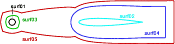
The instantaneous values for pressure and velocity are recorded from DES simulation on the surfaces extracted from finite volumes without interpolation. The surfaces around the rod and airfoil (surf03 - surf05) implicitly take the noise of sources based on turbulence inside the surface, known as quadrupole noise, into account. Owing to the symmetry of the rod-airfoil test case, the radiated sound for 60 observers is computed above the airfoil on a circle of radius R=1.85 m (see Fig. 1). All spectra are obtained by a FFT, with a length of 8192 points with 50 averagings and the use of a Hanning-window. This leads to a spectral resolution of $\Delta f \sim 24 ~Hz$. For meaningful comparisons with experimental and LES spectra of different frequency resolution, the Power Spectral Density (PSD) is used for comparison. The simulated span $L_{sim}= 3d$ is less than the span of the test configuration $L_{exp}= 30d$, so a level correction has been applied based on the work of Kato.

Figure 11: Comparison of different integration surfaces

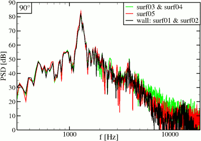
The acoustic results calculated for an observer on the afore mentioned circle $\Theta = 90$, are compared for rigid and penetrable integration surfaces based on k-ε-DES in Fig. 11. These are the obtained spectra of the complete rod-airfoil configuration based on the on-wall computations of the rod and airfoil (surf01 & surf02) as well as from the penetrable surfaces that separately surround the rod and airfoil (surf03 & surf04) and the surface surrounding the entire rod-airfoil configuration (surf05). As an exception, averaging and level correction as described above is not applied. Even though there is a slight difference between the integration surfaces for frequencies beyond 4 kHz and in the level of the main Strouhal peak. The obtained far-field spectra in general agree well with each other. The level of the main Strouhal peak is increased by 1-2 dB through use of the penetrable surfaces for the acoustic calculation.

Figure 12: Comparison of DES and LES to
measurements of Jacob for an observer
(R = 1.85 m) normal to the flow

Figure 13: Directivity plot of k-ε-DES
in comparison to measurements from Jacob (R = 1.85 m)

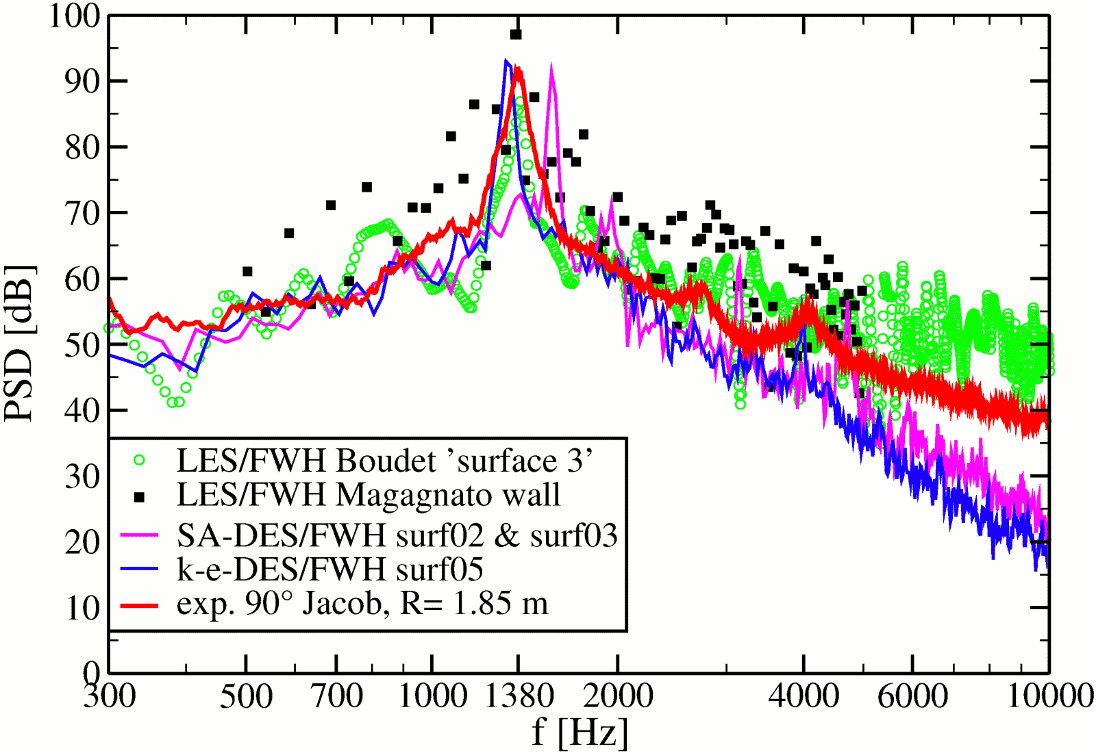
Figure 12 shows the DES/FWH results in comparison with measurements and LES computations for an observer in the direction of $\Theta = 90$. Both DES simulations are in very good agreement up to 4-5 kHz with the broadband spectrum based on measurements. The level of the main Strouhal peak is well estimated, but the SA-DES slightly overpredicts the frequency. Irrespective of the accuracy of the main peak, the ratio of frequencies between the main peak and the higher harmonic peaks coincides with experiment in all cases. As the frequency of the main Strouhal peak is well predicted by the LES/FWH of Boudet and Magagnato, the magnitude is slightly underpredicted by Boudet. The overpredicted levels and a large vertical spread of the LES data of Magagnato is observed in the whole frequency spectrum. The same problem is observed for the Boudet-LES data for frequencies beyond 4 kHz. The advantage of DES of lower computational costs allows to compute longer time-series for well-converged statistics and averaging in the acoustic data analysis. The presented DES simulations have shown to be capable of predicting the difficult low-frequency range together with a reduced vertical scatter at high frequencies. All computations shown the broadening of the main Strouhal peak.

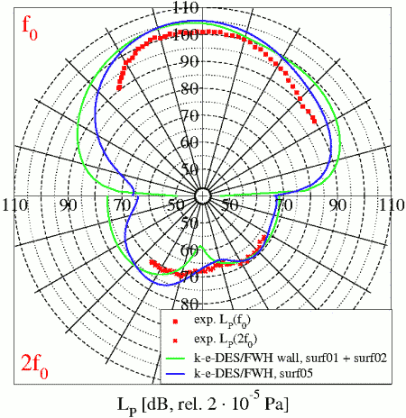
Finally, the directivity obtained from the favored k-ε-DES/FWH computations based on wall and a penetrable surface (surf05), respectively in comparison with the experiment are shown in Fig. 13. Depicted is in the upper half the directivity of the main Strouhal peak and the directivity of the double main frequency at the bottom. An excellent agreement is found between the computed directivity based on penetrable surface surf05 and the measurements, although a constant 3-4dB overprediction of the sound pressure level is observed at the main Strouhal peak in all measured directions. The corresponding directivity based on the solid-surface computations is less good, displaying also an incorrect qualatative behavior. The simulated directivity for the doubled basic frequency $2f_0$ is in good agreement to the measurements.