Aerodynamics

Rod-Airfoil configuration, Flow simulation & DES method

Figure 1: Rod-airfoil configuration.
A and B are the hot-wire measurements

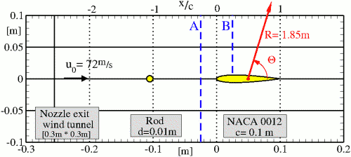
An experimental investigation of a rod-airfoil configuration was conducted at ECL. A symmetric NACA0012 airfoil (chord c=0.1 m) and a circular rod (d/c = 0.1) were placed in the potential core of the jet.

A complete description of the configuration and the measurements can be found in [Jacob et al.] and [Michard et al.].

The flow is computed numerically using StarCD^TM, a volume-based code solving the unsteady Reynolds-averaged Navier-Stokes equations (RANS) in an implicit manner, of first order in time and second order in space. All computations, except the preliminary two dimensional investigations, are compressible using an equation for total thermal enthalpy and the ideal gas equation $\varrho = p/RT$. The convective terms are approximated with second order central or upwind-biased, limited schemes of higher order (MARS). For the k-ε-DES a blending function [Travin et al.] for hybrid (MARS-central) numerical convection schemes is used to resolve the conflicting numerical requirements of LES and RANS regions. The grid is composed of about 1.9 million cells with 224 points around the rod and 344 points around the NACA0012 in circumferential direction. The normalized first cell spacing normal to the wall is y⁺ < 1.5, except in separation zones behind the rod. [2D slice of computational grid (PNG 330kB)]
The time step is set to $\Delta t = 5 \cdot 10^{-6} ~s$, leading to around 150 steps per shedding cycle. The preliminary 2D-URANS simulations used a time step of $\Delta t = 1 \cdot 10^{-5} ~s$. The number of time steps computed for statistics and acoustic output was 30000 for k-ε-DES , and 20000 for SA-DES, that corresponds to 200 and 150 shedding cycles, respectively.

The present investigation of broadband noise prediction is concerned with the influence of different approaches in turbulence modeling for the Detached Eddy Simulation approach (DES). This non-zonal, hybrid technique was introduced by Shur in 1997 in order to combine the strengths of RANS and LES. The fundamental advantages of this hybrid approach are manifest both in terms of computational costs and of accuracy in the prediction of complex wall bounded flows. Furthermore, the high performance of LES in the outer turbulent regions is maintained in the DES technique. The DES combines the URANS and LES by non-zonal blending. Near the wall a standard RANS model is used and in the outer, detached regions of the flow the RANS model operates as an LES-like sub-grid-scale (SGS) eddy viscosity model. This is achieved by modifying the relevant model transport equation to limit the eddy viscosity. The switching between the two methods is obtained by modification of the length scale $l_{turb}$ of the turbulence model. This length scale is compared with the local grid dimension $\Delta$, similar to an implicit filter in LES.

The method of modification of the transport equation is different for SA- and k-ε-DES. [Shur et al.]

Results and Discussion

Figure 3: Instantaneous vorticity iso-surface
a) SA-DES, b) k-ε-DES and c) LES from Boudet bottom

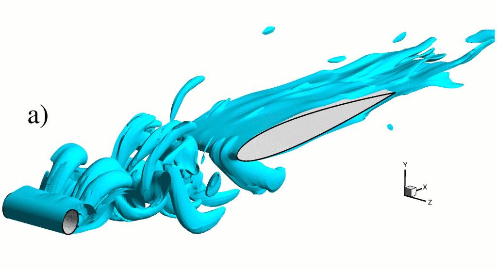
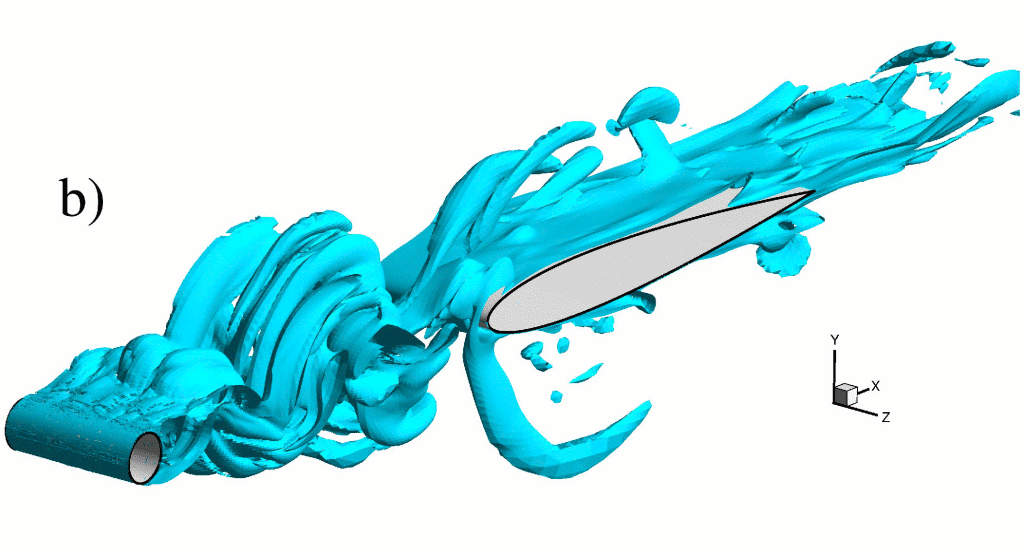
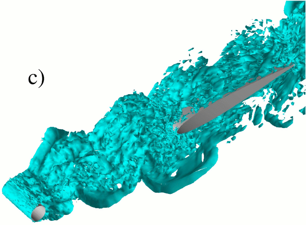
In order to give a qualitative overview of the 3D flow, snapshots of iso-surfaces of the vorticity are plotted in Fig. 3 for the SA- and k-ε-DES and LES. All cases show the fully-developed three dimensional flow, where the main shedding can be recognized by oscillations in the wake of the rod. Peak values of up to 40 m/s in the z-velocity component are observed for the DES calculations. Figure 3c shows a traditional LES result of Boudet for comparison. This LES additionally shows small turbulent eddys affecting the large-scale structures. This further indicates that the compared LES calculations clearly benefits from the use of much smaller time steps and higher order spacial and time discretization schemes by the resolution of smaller structures in the flow field.

The improved results of k-ε-DES compared to SA-DES is characterized by a general correct tendency in all statistical values. The statistics are given in Table 1, compared to values of LES and preliminary 2D-URANS investigations.

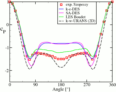
The mean pressure coefficient $c_p$ on the rod surface is shown in Fig. 4. The present DES and former LES computations are compared to the measurements of Szepessy, which are obtained for an isolated rod under the same flow conditions ($Re_d = 4 \cdot 10^4$). The k-ε-DES computation (blue line) is in a very good agreement with the experiment, except in the separation area where the pressure is over predicted. The incorrect prediction of the drag is due to a small secondary vortex oscillating on the rear surface of the cylinder, which is present in the simulation. The LES computation from Boudet also agrees with the experiment in the separated flow area. The SA-DES computation predicts nearly the same value for $c_p$ in the separated flow area as k-ε-DES . Fig. 4 shows also one result from a two-dimensional simulation, with a modified version of k-ω-turbulence model. The standard deviation of the fluctuating lift $c_{L_{rms}} = 1.14$ is over predicted, but the drag is close to the experimental data (2D k-ω-URANS: $c_{D_{rms}}= 0.19$ and $\overline{c_{D}} = 1.35$ ).

Table 1: Statistics and means for rod, $d= 0.01 ~m$, $Re_d=48000$

test case	St	$c_{L_{rms}}'$	$c_{D_{rms}}'$	$\overline{c_{D}}$
Szepessy	0.19	0.45-0.55	0.16	1.35
Schewe	0.185	0.45	0.22	1.1-1.2
SA-DES	0.217	0.34	0.05	0.77
k-ε-DES	0.185	0.42	0.03	0.81
LES Boudet	0.19	0.57	0.12	1.17
LES Magagnato	0.19-0.203	-	-	-
various 2D-URANS	0.24-0.26	0.41-1.34	0.02-0.32	0.75-1.38

Figure 4: Mean pressure coefficient on the rod.
Zero angle is defined by stagnation point.
Measurements from Szepessy. LES from Boudet,
SA-DES, k-ε-DES and 2D k-ω-URANS

Figure 5: Mean velocity field for SA-DES (top),
k-ε-DES (bottom) turbulence model.

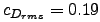
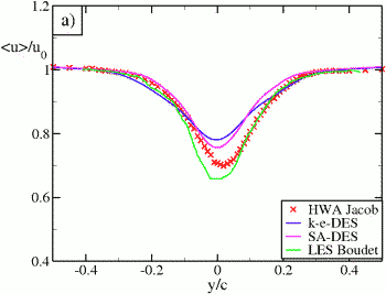
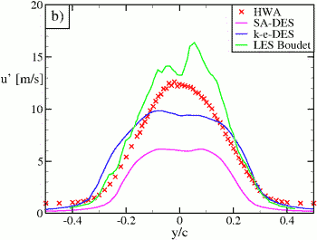
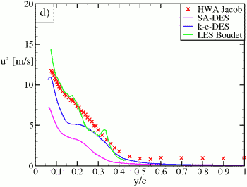
The mean and fluctuating velocities in the stream wise direction are compared to hot-wire anemometry (HWA) measurements on Fig. 6 for the cross sections A and B (shown in Fig. 1). Figure 6a and b summarizes the results for section A, which is located 1/4 chord length upstream of the airfoil leading edge. The mean velocity on the left side and the rms-value of fluctuating velocity on the right side are well predicted by LES [Boudet et al.] and slightly under predicted by k-ε-DES. SA-DES clearly under predicts the values for fluctuating velocity. Section B, which is located above the airfoil, shows the same behavior. Additionally, LES results from Magagnato are shown in Fig. 6c for the mean velocity. DES is in good agreement with LES simulation and experiment, except in the near-wall region.

In order to characterize the unsteady simulated flow the spectra based on unsteady velocity at Position x/c = 0.25 (cross-section B), y/c = 0.3 are shown in comparison with the hot-wire anemometry data. The k-ε-DES and LES [Boudet et al.] predict the levels over a wide frequency range accurately and the peak of the shedding frequency is in agreement to the experiment. The LES results at high frequencies up to 12 kHz are in good agreement with the experiment, above this an abrupt cut-off is observed due to the sub grid-scale filter. The DES simulations show a smooth decay above a frequency of 3-5 kHz. The observed level of SA-DES is around 5-8 dB below the experimental data. 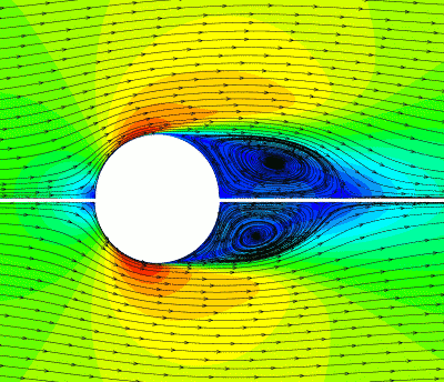According to that, Fig. 5 shows a comparison of the mean velocity field for SA-DES at the top and for k-ε-DES at the bottom.

Figure 6: Mean and RMS of velocities at x/c = -0.25d (top) and x/c = 0.25d (bottom).
Hot-wire anemometry measurements from Jacob, LES from Boudet, k-ε-DES and SA-DES.
Also at position x/c = -0.25d, mean values of LES from Magagnato

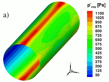
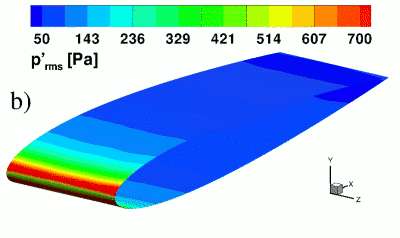
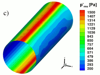
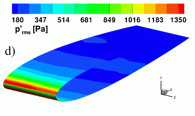
The rms-value of pressure perturbation on the surface of the rod and airfoil for the two DES computations is shown in Fig. 7. The main dipole characteristic of the rod becomes clearly visible in both simulations. Even though the k-ε-DES shows stronger fluctuations at upper and lower side of the rod, the wake fluctuations are weaker than that of the SA-DES. That indicates a shorter wake in case of the SA-DES which explains the the over predicted Strouhal frequency. For the airfoil the strongest perturbations are observed near its leading edge, where the rod-created vortexes impinge on its surface. Again the fluctuations are stronger for k-ε-DES. 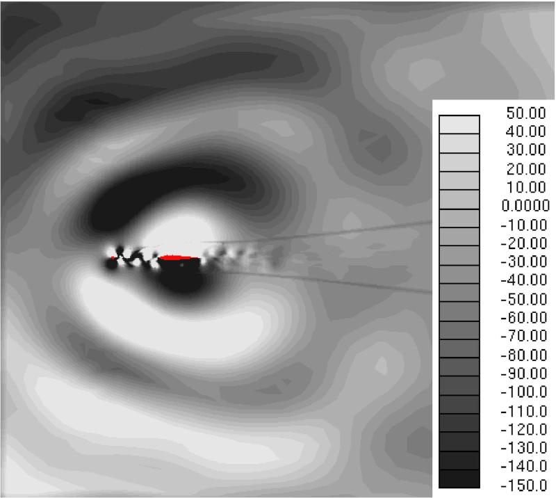Additionally in Fig. 8 the pressure perturbation in the near-field of the configuration is shown. This shows waves traveling away from the rod-airfoil-configuration. The complete configuration carries a dipole characteristic, which becomes obvious from the dominating wave structures.

Figure 7: Rms value of surface pressure perturbation of rod
and NACA0012. a,b) SA-DES and c,d) k-ε-DES
+ Animation for k-ε- DES model > Rod (2Mb) and NACA0012 (2.4Mb).

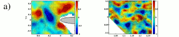
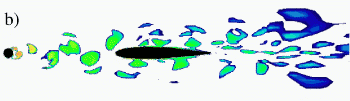
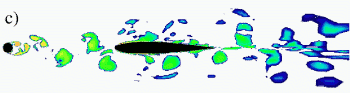
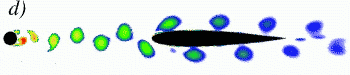
Finally, a comparison of the instantaneous vorticity flow field obtained from PIV, DES and URANS is made in Fig. 9 in order to illustrate the variety and complexity of the flow. In the upper part contours of the $G_2$-criterion based on the POD analysis of PIV measurements upstream of the leading edge and downstream of the trailing edge are shown. The POD analysis evaluates the eigenvalues of instantaneous velocity fields to detect the main and secondary vortex structures in the flow field, these are compared with contours of the $\lambda _2$-criterion [Jeong et al.] for SA-DES, k-ε-DES and 2D SA-URANS (top to bottom). This criterion evaluates the eigenvalues of the strain tensor to detect the main vortex structures, and is comparable to the afore mentioned $G_2$-criterion. The $\lambda _2$-criterion evaluates only the magnitude of the eigenvalue, so there is no possibility to separate the swirl direction. The URANS simulation is purely periodic. The main vorticities are propagated downstream and dissipated. The constant z-slices of both DES simulations show regular vortex structures near the rod that are deformed to irregular patterns when they are convected downstream, owing to the redistribution of the turbulent kinetic energy in the z-direction. The small vortex structures downstream of the trailing edge predicted by DES are in good agreement with the PIV snapshots.

Figure 8: Pressure perturbation in the near-field of Rod and NACA0012 of k-ε-DES

Figure 9: Comparison of POD ($G_2$) based on experimental data (PIV) (a) and $\lambda _2$-criteria of SA-DES (b), k-ε-DES (c) and 2D SA-URANS (d) to detect the main vortex structures in the flow field