


Next: Selected validational testcases and
Up: Eddy-Viscosity Transport Model
Previous: Eddy-Viscosity Transport Model
Amongst the various recent publications on one-equation models,
Menters [2] rigorous derivation of a generic
one-equation model casted in terms of a transport equation for the eddy-viscosity  is, perhaps, the most instructive.
Based on the application of local-equilibrium assumptions
to a two-equation - e.g.
is, perhaps, the most instructive.
Based on the application of local-equilibrium assumptions
to a two-equation - e.g.
 - model,
Menters approach provides a keen insight into the one-equation modeling framework,
in particular the related coefficients.
The procedure reveals that the four most influential production and destruction terms of the two-equation
approach collapse into a single production-type term in the one-equation framework, viz.
- model,
Menters approach provides a keen insight into the one-equation modeling framework,
in particular the related coefficients.
The procedure reveals that the four most influential production and destruction terms of the two-equation
approach collapse into a single production-type term in the one-equation framework, viz.
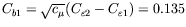
The coefficient  is thus crucial to the model's predictive performance.
As indicated by eq. (5), is a function of the strain rate
and model coefficients.
Substituting the employed coefficients of the background
turbulence model
by
is thus crucial to the model's predictive performance.
As indicated by eq. (5), is a function of the strain rate
and model coefficients.
Substituting the employed coefficients of the background
turbulence model
by
 and
and
 ,
additionally employing
,
additionally employing
 one obtains
 , which
is close to the original SA model (
, which
is close to the original SA model (
 ).
Both expressions,
).
Both expressions,
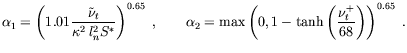
 and the anisotropy parameter
  ,
are itself a function of strain and rotation rate invariants. In general, they both tend
to decrease with an increase of strain, which motivates the following modification of the standard
coefficient :
,
are itself a function of strain and rotation rate invariants. In general, they both tend
to decrease with an increase of strain, which motivates the following modification of the standard
coefficient :
 |
|
|
(6) |
Due to the lack of an individual length-scale the approach relies on some heuristics
based on the comparison of a mixing-length related eddy-viscosity with the value obtained
from the solution of the transport equation. The modification
 primarily causes
a reduction of production for excessive strains via
primarily causes
a reduction of production for excessive strains via  . Additionally, undesirable wall-damping
is suppressed by the inclusion of
. Additionally, undesirable wall-damping
is suppressed by the inclusion of  .
The limitation of
.
The limitation of  are necessary due to the proportionality of
 and , i.e.
a decreasing
causes a decreasing .
Since it is closely related to the destruction parameter
and , i.e.
a decreasing
causes a decreasing .
Since it is closely related to the destruction parameter  ,
the modification of
,
the modification of
 represents a cross-term between
production and destruction.
represents a cross-term between
production and destruction.
Next: Selected validational testcases and
Up: Eddy-Viscosity Transport Model
Previous: Eddy-Viscosity Transport Model
Markus Schatz
2004-02-10