


Next: Production-Term Modification
Up: J26222
Previous: Introduction
The proposed Strain-Adaptive Linear Spalart-Allmaras (SALSA) model
complies in most parts with the original SA model.
The present model is based on the eddy-viscosity principle for weakly
compressible media with negligible density fluctuations, viz.
 |
|
|
(1) |
where  ,
,
 and
and
 denote to the mean velocity,
kinematic Reynolds stresses and turbulence energy, respectively.
The eddy-viscosity principle (1) is supplemented by a transport equation
for the undamped turbulent (eddy) viscosity
denote to the mean velocity,
kinematic Reynolds stresses and turbulence energy, respectively.
The eddy-viscosity principle (1) is supplemented by a transport equation
for the undamped turbulent (eddy) viscosity
 defined in eq. (2)
![$\displaystyle \frac{ D\tilde\nu_t}{ Dt}
-\frac{\partial }{\partial x_k} \left[ ...
...}{Pr_{\tilde\nu_t}} \right] \frac{\tilde\nu_t ^2}{l_n ^2}}_{\rm Dissipation}\:.$](img16.png) |
|
|
(2) |
The employed damping-functions and coefficients read as follows:
Here,  is the wall-normal distance determined in a customary manner.
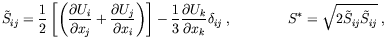
The definition of the effective velocity gradient
is the wall-normal distance determined in a customary manner.
The definition of the effective velocity gradient  is given by
The choice of the near-wall parameter  follows a route outlined by Edwards [3]
and is motivated by the more robust behaviour experienced for complex industrial applications.
It should be noted, that the adopted near-wall model slightly alters the predicted skin friction
in equilibrium flows.
For a flat-plate boundary layer at
follows a route outlined by Edwards [3]
and is motivated by the more robust behaviour experienced for complex industrial applications.
It should be noted, that the adopted near-wall model slightly alters the predicted skin friction
in equilibrium flows.
For a flat-plate boundary layer at
 the predicted
shape factor
the predicted
shape factor  increases by 1.8 % and the skin friction decreases by the same amount when compared to the SA model.
The specific closure of the production-term
 is outlined in the next section.
Subsections
Next: Production-Term Modification
Up: J26222
Previous: Introduction
Markus Schatz
2004-02-10
![$\displaystyle f_{\nu 1} = \frac{(\nu_t^+)^3}{C_{\nu 1}^3 + (\nu_t^+)^3} \: ,\qq...
...ight]^{1/6} \:, \qquad
g = r \left[ 1+ C_{w2} \left(r^5 -1 \right) \right] \: ,$](img17.png)