|
|
|
 =0). A low order CFD Euler solution was used to compute the mean flowfield as a basis for the
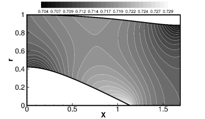
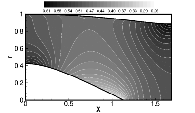
sound propagation simulation. The calculated mean flowfield is shown in Fig. 4 where M0=-0.5 is an averaged mean flow Mach number at the source plane x=0. It should be pointed
out that the entropy distribution generated by CFD is not exactly constant due to numerical errors especially
around the spinner tip and duct lip regions. However, these non-homentropic regions are very limited and the
disturbance in the speed of sound
=0). A low order CFD Euler solution was used to compute the mean flowfield as a basis for the
sound propagation simulation. The calculated mean flowfield is shown in Fig. 4 where M0=-0.5 is an averaged mean flow Mach number at the source plane x=0. It should be pointed
out that the entropy distribution generated by CFD is not exactly constant due to numerical errors especially
around the spinner tip and duct lip regions. However, these non-homentropic regions are very limited and the
disturbance in the speed of sound
 is first order with respect to the perturbation quantities.
The products of the perturbation quantities and the disturbance of homentropy are therefore second order.
The entire mean flowfield can be approximated as homentropic which is consistent with the acoustic computations.
is first order with respect to the perturbation quantities.
The products of the perturbation quantities and the disturbance of homentropy are therefore second order.
The entire mean flowfield can be approximated as homentropic which is consistent with the acoustic computations.
Because of the differing requirements for CFD and CAA calculations, both procedures need different grids. This requires an interpolation of the mean flowfield from the CFD grid to the CAA grid. A routine for this interpolation has been provided by DLR[19]. Fig. 4 shows that the mean flowfield varies in both the radial and axial directions, even at the source plane x=0.
There are differences in the mean flow solution among the CAA, FEM and MS methods.
The FEM computations are based on a 2D potential mean flow which is very close to that used in
the CAA computations. The CAA mean flow is non-uniform throughout the duct, however,
the FEM and MS mean flow velocities are uniform at the source plane x=0.
Unlike the CAA and FEM methods, the mean flow in MS is based on a quasi one-dimensional solution,
which is consistent with the multiple scales approximation.
It is expected that these differences should result in deviations in the acoustic computation results.
|
|
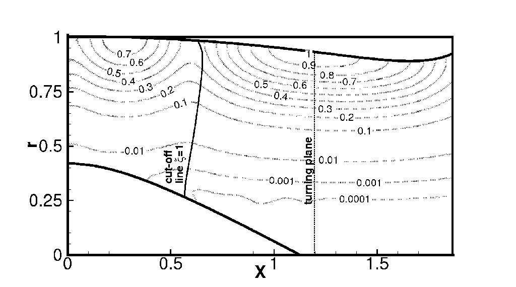
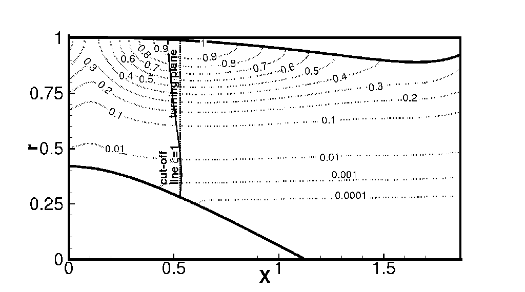
Fig. 5 shows the one-dimensional potential mean flow, which is calculated for the same duct geometry. In order to compare the difference mean flow assumptions, with respect to their influence on the cut-on/cut-off transition,
the two different mean flow profiles are compared in the following section.
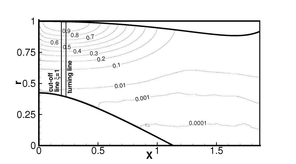
To show the capability of the proposed CAA procedure, the hard walled cuton and cutoff transition phenomena is investigated for the same axisymmetric aero-engine inlet duct.
The cuton and cutoff transition of a mode in a hard-wall flow duct is also known as a turning point problem. It was
studied by Nayfeh & Telionis[20] for the no-flow case and was recently extended to include flow effects by
Rienstra[21]. In the case of no-flow, the transition or turning points are solely determined by the variation of
duct geometry which is mathematically described by the cutoff ratio ξ. The portions of the duct for which ω>μmn
are defined as cuton regions while those for which ω<μmn where the imaginary part of the axial wave number is non-zero
are known as cutoff regions. The axial positions at which ω=μmn are called the transition or turning points.
A direct practical application is to reduce the acoustic energy in a duct by gradually decreasing and then increasing
its cross-sectional area[20], as the imaginary part of the wave number is connected to a
decaying amplitude of the related mode.
Rienstra's study[21] further showed that the usual turning point behavior could also be found
in a slowly varying hard-walled duct with irrotational isentropic mean flow. In addition to the geometric effect, the mean flow
effect must be included for cases incorporating a mean flow. Theoretically the turning plane is located at the position where
 .
.
The decaying mode can propagate only for cases with mean flow. In the no-flow case, the axial wave number is zero at the turning plane which is related to an infinite axial wavelength and the acoustic wave will not propagate forward with a wavefront normal to the duct wall. Due to the conservation of the acoustic energy in case of homentropic mean flow, the turning plane must excite a reflected wave transferring the energy backward to the sound source region. With mean flow, there is a transmitted cutoff wave with wave number k=-ωMx. The reflected and incoming waves both have positive wavenumbers related to phase velocities opposed to the flow direction. Nonetheless, the group velocity associated with energy transport is only positive for the incoming wave. Therefore a pattern of positive and negative interference between the incoming and reflected waves should be observed for each turning point. The sound source has to be non-reflective to the reflected wave in this case.
|
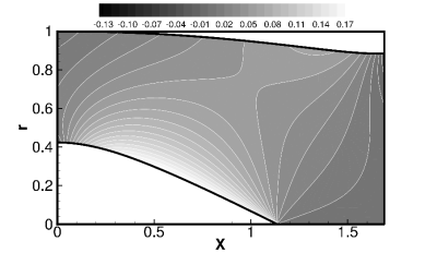
Furthermore, a cuton and cutoff transition case is shown in Fig. 7 based on an Euler mean flow (as shown in Fig. 4 with M0=-0.5) for m=10, n=1, ω=11.129. The variation of the flow is rather strong especially around the spinner and the lip region which violates the assumption of uniform mean flow. The approximated turning plane based on the equation for the complex wave number k is located at the x≈0.6. However, the CAA calculated results show a standing wave pattern at x<1.2 and a decaying wave pattern from x>1.2. This is done in spite of the rough approximation of the real flow conditions due to the variable geometry. This means that the CAA calculated turning plane is roughly located at x=1.2, while the analytical solution locates it at x≈0.6, in a radially relatively constant mean flow. The conclusion is therefore that the shown radial variation of the flow in a real engine inlet has a vital influence on the turning behavior.
|
|
Considering the available theoretical studies for the no-flow case by Nayfeh & Telionis[20] and for the irrotational isentropic mean flow case using the slowly variable duct approximations by Rienstra[21], the investigation in this paper provides an additional understanding about the cuton and cutoff transition behavior in complex mean flow ducts. In particular, the physical correctness of the mean flow is crucial for the accurate prediction of the turning plane.