Verification and Validation

The Mean Flowfield is shown on the next site. >

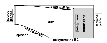
Figure 1: BCs for a generic aeroengine inlet geometry.

The necessary appropriate boundary conditions for both the circular and annular ducts are merely simplifications from the arrangement for a complicated aero-engine inlet duct geometry as sketched in Fig.1. In both cases, the sound sources are excited against the uniform mean flow of M₀=-0.5. Since the cross section and mean flow are constant for both validation cases, there are no reflection waves from the inflow regions. Hence the numerical results can be compared with analytical upstream wave solutions.

A comparison between the CAA, FEM and MS solutions

Large number of numerical tests have been carried out with parameter variations of m, n, ω and M₀. In the interests of brevity, only two typical cases are presented below.

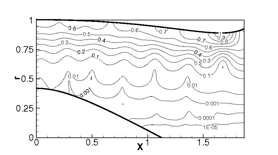
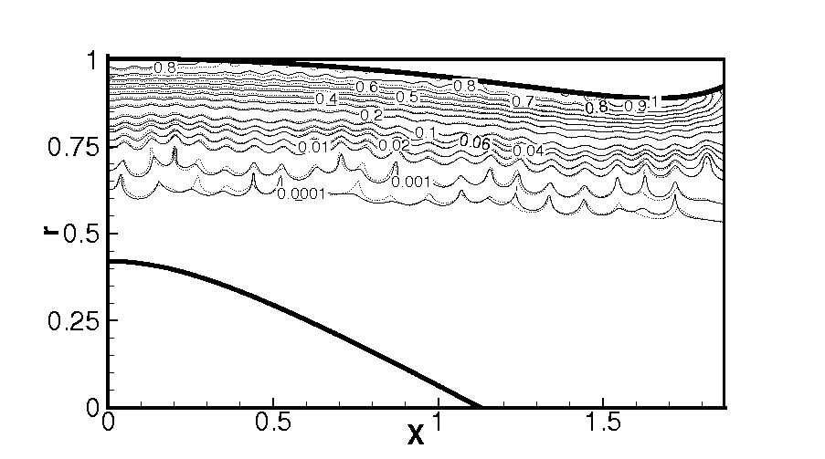
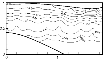
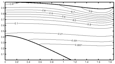
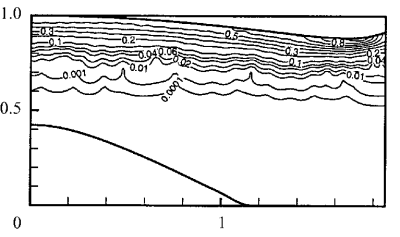
Figure 2: Normalized pressure contures (M₀=-0.5, m=10, n=1, ω=16). Top down: CAA, FEM, and MS.

First, the numerical results for the m=10, n=1, ω=16 case with mean flow at M₀=-0.5 is presented in Fig. 2 and compared with the solutions of the FEM and MS methods^[10]. The main pattern of the CAA results agree well with the FEM and MS solutions. However, the CAA solutions are much closer to the FEM solutions. There are two main reasons for this. Firstly both the CAA and FEM numerical methods permit the propagation of many modes and scattering is incorporated in the numerical solutions, whereas the MS method assumes that a single mode does not scatter into other modes in the gradually varying duct. The cutoff ratio, ξ is approximately 1.57 at x=0 for the case of m=10, n=1, ω=16, and M₀=-0.5. Theoretically, the second radial mode (m=10, n=2, ω=16, M₀=-0.5) is also cuton with ξ≈1.124 at x=0. This implies that the second radial mode is capable of being scattered and of interfering with the excited first radial mode in both the CAA and FEM solutions. However, no interference between modes should occur in the MS solution due to the WKB assumption of each mode in the slowly varying duct. The second reason is that both the CAA and FEM solutions include the reflected modal amplitudes from the duct and mean flow variations, particularly from the duct lip and inlet plane regions. But the left and right running waves have been explicitly given in the MS solution, which has excluded the reflection characteristics apparent in the real physics. Therefore the CAA and FEM solutions have clear interference patterns and some visible wiggles whereas the MS exhibits very smooth contours. Higher radial modes can be observed for both FEM and CAA especially around x=0.2, 1.0, and 1.6, where a higher pressure amplitude at the casing appears together with a minimum value at around x=0.5.

Comparing carefully the CAA and FEM solutions, some differences can be observed near the hard-wall boundary region, particularly in the lip and spinner tip regions. This deviation is mainly attributed to the different mean flows used in the respective calculations. Compared with mean flow used in the FEM calculations^[10], the mean flow used in the CAA calculations have stronger radial and axial variations . It would be possible to use an equivalent mean flow for exact comparison, however it's not absolutely required since the observed difference between the CAA and FEM methods are already very minimal.

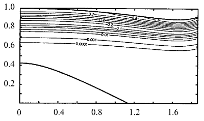
Figure 3: Normalized pressure contures (M₀=-0.5, m=40, n=1, ω=50). Top down: CAA, FEM, and MS. In the CAA results, the solid and dotted lines were calculated based on the coarse and refined grids, respectively.

Variations in frequency ω and the azimuthal mode number m can lead to different propagation patterns. Given a fixed azimuthal mode number m and radial mode number n, the cutoff ratio ξ at the source plane x=0 will increase with increasing frequency. To give an example, ξ will be increased to about 4.905 if ω is set to 50 for the case of m=10, n=1, M₀=-0.5. Then 11 radial modes will be cuton and the first radial mode will interfere with 10 scattered higher radial modes. Several CAA solutions have been compared with the FEM and MS solutions with a good agreement and will not be presented here.

With respected to an increase in azimuthal mode number m, the radial wave number of the primary first radial mode will be increased. Fig. 3 shows a comparison of results for m=40, n=1, ω=50 and M₀=-0.5. In this case, the cutoff ratio ξ at x=0 is about 1.35 for the first radial mode. Theoretically the first three radial modes are cuton. In Fig. 3, the CAA results were calculated based on both the coarse mesh (solid lines, with 451 × 151 grid points) and the refined mesh (dotted lines, with 901 × 301 grid points). Both the contour lines agree well, only very small differences can be observed at the very low amplitude regions. The numerical solutions (CAA, FEM) for m=40 agree better with the MS solutions compared with the agreement at the lower azimuthal mode case of m=10. However, wiggles in the CAA and FEM solutions are still visible because of scattering of higher radial modes.

In general, the CAA solutions agree well with the FEM and MS solutions. This indicates that the proposed CAA procedure has comparable properties for predicting the sound propagation in ducts with complex geometry and flow physics, while employing a different numerical method with different than FEM and MS assumptions in the solution.