Validation and Application

Generic Bell Mouth Intake

To demonstrate the capability of the 3D axisymmetric CAA procedure, a generic bell-mouth inlet has been selected for benchmarking [Li et al. (2002)]. A sketch of the inlet geometry and the far-field microphone positions is depicted in Figure 3.

Figure 3: Sketch of the inlet geometry and far-field microphone positions

Figure 4: Instantaneous pressure contours, m=4 mode for M=-0.039

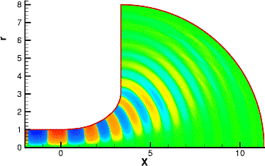
To model the sound source, the analytical solution for a circular duct is used. With this model, several propagating azimuthal modes known from experiment are calculated with normalized amplitudes. In Figure 4 the instantaneous pressure contours of the m=4 mode for a mean flow Mach number of M=-0.039 from the 2D calculation is shown. The diffraction of the propagating waves can clearly be observed.

To obtain the 3D sound field the normalized 2D solutions for the modes are scaled by their measured amplitude and superposed with respect to their phase. This procedure is used because the 2D modal results only depend on the inlet geometry, the mean flow, and the blade passing frequency and its harmonics. Therefore, for varying sound sources and unchanged inlet geometry and mean flow, only the post processing has to be repeated. This approach significantly reduces the numerical effort required to model changes of the source, such as rotor and stator geometries.

Figure 5: Instantaneous pressure contours of recomposed 3D sound field for M=-0.039

The recomposed 3D sound field of the generic bell-mouth intake at M=-0.039 for the 1st blade passage frequency (BPF) is shown in Figure 5. On the left a cut 3D view is plotted. The upper right shows a front view, and the lower right provides a side view. It can be observed that the employed approach can yield 3D truly asymmetric results.

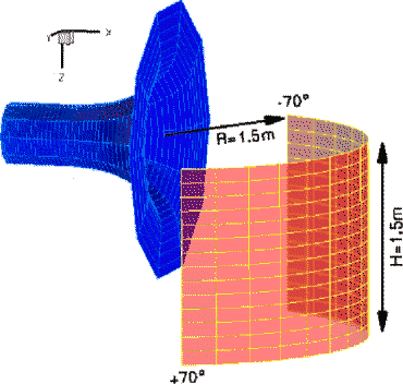
The far-field directivity is calculated on a cylinder segment with radius r=1.5m from -70° to 70° in front of the intake (see Fig. 3).

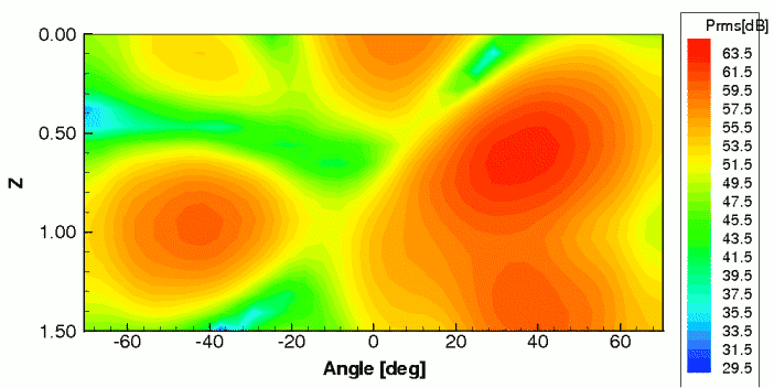
The directivity plot from the numerical solution is shown in Figure 6. A comparison with measured data shows a good qualitative agreement between simulation and experiment.

Figure 6: Directivity plot for the generic bell-mouth intake

Axisymmetrical Duct With Swirling Mean Flow

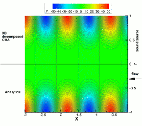
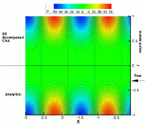
The validation for the swirling flow is based on an analytical solution modeling the noise propagation of each radial mode within a solid-body-rotational, uniform, subsonic mean flow in a straight circular duct. The solution is found by neglecting the Coriolis force, and therefore it is restricted to low angular velocities. The mean flow field is assumed to be uniform except for the azimuthal component. This solution is used for validation and as a sound source.

Figure 7: Instantaneous pressure contours of the m=4 mode for M=-0.5 at Ω=-0.3;0.0;+0.3

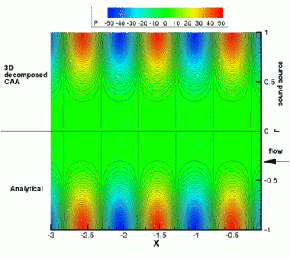
Fig. 7 shows a moderate effect of swirl on the axial wave-length at low angular velocities of Ω= ± 0.3 in comparison to the case without swirl, which was also computed using this approach. The numerical solution given in the upper part of each picture is in good agreement with the analytical solution given below. The peak pressure amplitude error is about 1% of the initial amplitude. At higher rotation speeds and for higher modes the azimuthal mode propagating with the swirl can become cut-off with exponential axial decay, while the counter-rotating mode remains cut-on in the swirl flow.

In general this effect is crucial for swirling flow at high speeds, as it can be found in the gap between the rotor and stator of the bypass duct, as well as in the whole bypass duct in several flight situations. The effect of variable cross section and of the nozzle interior will be the subject of future studies.

Scarfed Inlet

In addition to the control of noise generation, an equally important task is to control noise propagation and radiation into the far-field. Due to weight limits, it has becomes difficult to achieve further noise reduction using acoustic liners. An alternative technology considered in recent years is to use negatively scarfed intakes. Conventionally, positively scarfed nacelles are used on commercial airliners for aerodynamic reasons. The basic idea of the negative scarfing is to reduce the sound intensity toward the ground at the expense of increasing the sound intensity toward the sky.

The main objective in this case is to investigate the scarfing effects on sound radiation from duct intakes. To simplify this complex problem, the nonlinear effects have not been considered. A family of negatively scarfed intakes are evaluated with three scarfing angles (-5°,-15°,-25°)for zero mean flow [Li et al. (2003)].

An acoustic mode is excited at the source region as m=26, n=1, k=32.8. To meet the resolution requirements of the CAA approach a block structured body fitted grid with approximately 7 million grid points is used.

Figure 8: Instantaneous pressure contours of the acoustic mode propagation and radiation from a scarfed intake (-15°) for m=26, n=1, k=32.8, M=0.0.

[3D Cut] 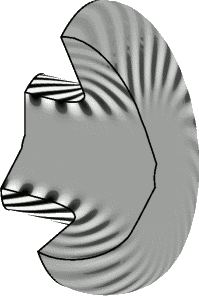[Front View]

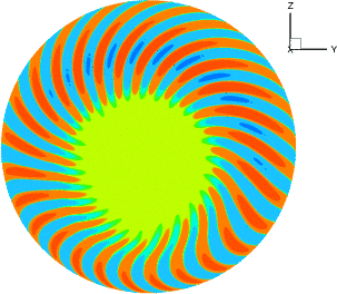
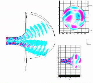
Fig. 8(a) shows instantaneous pressure contours for a negatively scarfed intake (-15°) at m=26, n=1, k=32.8, M=0.0. The acoustic mode propagation and radiation pattern is very clear. The detailed radiation pattern in the far-field boundary of the CAA computational domain is shown in Fig. 8(b) for γ=-15° which further indicates that there is a slight shift in the clockwise direction due to the rotation (-mΦ) of the excited sound mode.

Figure 9: A comparison results of far-field directivities for different scarfing angle intakes with m=26, n=1, k=32.8, M=0.0.

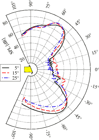
The CAA computations are carried out until the perturbation quantities become periodic. For the far-field integration, the periodic solution of the perturbation quantities is used. To determine the time derivatives, all the information on the FW-H surface is then sampled for more than one period for far-field integration. The far-field observers are located at 39.5 duct radii from the center of the intake cross sections. Fig. 9 shows the calculated far-field directivities of the three negatively scarfed intakes. These results clearly indicate the effectiveness of the scarf at reflecting more sound upward, thereby reducing the sound radiation towards the ground. For γ=-15°, the peak sound pressure level in the shadow of the scarfed intake is nearly 4dB less than it is above the scarfed intake. With an increased scarf angle of γ=-25°, the peak noise reduction can reach 10dB. However, only 1dB benefit can be achieved for a small scarf angle of γ=-5°. As the scarf angle further increases, the main radiation lobes shift gradually from the beneath to above the scarf. These results are in agreement with the experiments of Baker & Bewick and Clark et al..