A two-dimensional sail in turbulent flow
in
Abstract
The two-dimensional, incompressible flow at Reynolds number
based on chord length of
![]() around an inextensible, massless sail (flexible membrane airfoil)
with varying excess length is examined solving the Reynolds-Averaged
Navier-Stokes (RANS) equations on computational grids deforming according to the sail movement.
The grid deformation is computed using the same numerical procedure solving the basic
equations of displacements for an isotropic, linearly elastic continuum.
Results are presented for fully turbulent conditions employing closure models of
different degree of complexity in comparison with experimental and analytical results
obtained from literature. The sail is modelled as a chain with frictionless hinges.
Good agreement can be found for low angle of attack and small excess length.
However, for higher angle of attack, approaching onset of separation and beyond,
the predictive accuracy varies significantly with the representation of
turbulence in conjunction with strong unsteady phenomena.
around an inextensible, massless sail (flexible membrane airfoil)
with varying excess length is examined solving the Reynolds-Averaged
Navier-Stokes (RANS) equations on computational grids deforming according to the sail movement.
The grid deformation is computed using the same numerical procedure solving the basic
equations of displacements for an isotropic, linearly elastic continuum.
Results are presented for fully turbulent conditions employing closure models of
different degree of complexity in comparison with experimental and analytical results
obtained from literature. The sail is modelled as a chain with frictionless hinges.
Good agreement can be found for low angle of attack and small excess length.
However, for higher angle of attack, approaching onset of separation and beyond,
the predictive accuracy varies significantly with the representation of
turbulence in conjunction with strong unsteady phenomena.
1 Introduction
Only recently the turbulent viscous flow equations have been
introduced as the fluid dynamic model in sail or membrane airfoil theory.
An advanced study of flexible, massless membrane wing aerodynamics
incorporating the RANS equations has been presented in Smith, Shyy, [1]
Unlike an airfoil which is usually regarded as a rigid 2D structure, the sail shape is a
function of both incidence and Reynolds number in which the shape itself
interacts with the pressure distribution in a rather complicated manner.
A hysteresis in aerodynamic characteristics is observed since there are two equilibria
at small angles of attack, i.e., the sail snaps through at
a certain angle of attack. However, snapping through could not
yet be computed due to the fact that the sail shape becomes highly instable and
the grid deformation very large.
There are several references for experimental results, e.g. Greenhalgh, Curtiss, Smith, [2], which will be taken for comparison, and a variety of theoretical investigations concerning membrane airfoil or sail theory exist, cf. [1].
The computation of turbulent flow around a flexible 2D sail poses a challenge for the flow solver as well as the structural-mechanics solver, since the simulation has to be time-accurate on a domain with moving boundaries. The prediction of the aerodynamic forces has to be as exact as possible in order to allow for a realistic representation of the sail shape that deforms according to these loads. As classical inviscid theory only holds for small ranges of angles of incidence with small excess lengths, the application of RANS methods becomes necessary for this task.
A chain model as given in de Matteis, de Socio, [3] is considered for the sail in conjunction with a RANS method instead of the sail equation that is usually used.
2 Description of Method
2.1 Fluid Mechanics
For the computation of the 2D flow around the sail an in-house
finite-volume (FV) method is used, which is based on an implicit procedure of
second order accuracy in time and space. Due to its fully implicit scheme, true time steps are
possible and steady flow simulations are unconditionally stable.
Moreover, this permits an unlimited variation of the time-step size.
Complex two-dimensional geometries and local mesh refinements can be
resolved by semi-structured grids, i.e. using hanging
nodes, on the basis of general curvilinear coordinates.
Moving meshes are implemented based upon the space-conservation law,
such that (forced) unsteadiness caused by moving boundaries can be captured.
The cartesian tensor components as well as all scalar
variables are stored in the control-volume centers. Diffusive terms are
approximated applying central difference schemes whereas convective
terms are approximated by upwind biased, bounded, monotonic functions of higher order,
Lien, Leschziner, [4].
The governing equations of the incompressible mean flow field,
the continuity equation and the transport equation(s) for turbulent quantities
are solved sequentially.
The solution is iterated to convergence using a compressible (all-speed)
pressure correction scheme of the SIMPLE type, Patankar, [5].
Introducing apparent pressures and viscosities, a generalised
Rhie & Chow interpolation avoids an odd-even decoupling of pressure, velocity, and
Reynolds stress
![]() , Obi, Peric, Scheurer, [6].
, Obi, Peric, Scheurer, [6].
The computational modelling of turbulent effects is based on
a variety of models featuring different degrees of complexity
to compute the Reynolds stresses arising in the averaging process.
Amongst the many implemented modelling practices are standard isotropic
Boussinesq-viscosity approaches employing either one or two additional transport equations
(
![]() ,
, ![]() ).
Moreover,
their extension to non-linear constitutive stress-strain
relations, as well as (non-linear) full Reynolds-stress transport models are available,
Rung, Lübcke, Xue, Thiele, Fu, [7].
In the present study, however, attention is restricted to the assessment of one- and two-
equation models: the standard (SA) and a modified (SALSA)
Spalart-Allmaras one-equation model,
and only two different
).
Moreover,
their extension to non-linear constitutive stress-strain
relations, as well as (non-linear) full Reynolds-stress transport models are available,
Rung, Lübcke, Xue, Thiele, Fu, [7].
In the present study, however, attention is restricted to the assessment of one- and two-
equation models: the standard (SA) and a modified (SALSA)
Spalart-Allmaras one-equation model,
and only two different ![]() two-equation models in comparison,
Rung, Thiele, [8],
because turbulence models of higher order did not show better results.
two-equation models in comparison,
Rung, Thiele, [8],
because turbulence models of higher order did not show better results.
Due to the implementation of grid fluxes arising from the formulation of transport equations on moving grids, the step from grids moving in a rigid-body manner to deforming grids does not require any changes in the part of the code solving the equations for the fluid.
2.2 Structure Mechanics
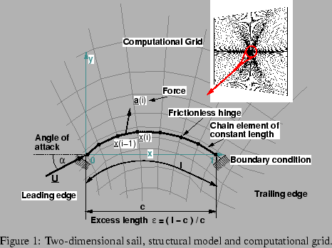
2.2.1 Sail
The model presented in this paper describes the behaviour of an inextensible, massless sail using
the structural model of a chain given in de Matteis, de Socio, [3].
This description was preferred in the beginning since an analytical function
for the membrane shape as in the sail equation does not easily allow for a
computation of the exact movement of the sail's material points.
Equilibrium of forces is evaluated at each grid node of the sail, see fig. 1,
leading to the following equation:
 |
(1) |
![$\displaystyle 0 = \big[ \frac{1}{2} l(i) \underline{a}(i) + \underline{F} (i) \big] \times \big[\underline{x}(i)-\underline{x}(i-1)\big]\;.$](img13.png) |
(2) |
Note that there are no time dependent terms included, thus inertia and damping are completely
neglected in the structure mechanics. This simplification has become necessary due to a
lack of experimental data concerning mass distribution and structural damping.
However, the iterative procedure to converge the solution
of these equations has to be started with a relaxation factor of ![]() that can slowly be raised each step
up to a maximum of 0.5.
that can slowly be raised each step
up to a maximum of 0.5.
Solving the sail equation
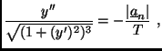 |
(3) |
2.2.2 Computational Grid
The starting point for the grid-deformation method is the momentum conservation equation
valid for a solid body in steady state without any volume loads:
 |
(4) |
Assuming ideally linearly elastic material, the stress-strain relation becomes
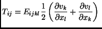 |
(5) |
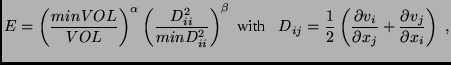
It has to be remarked, that although the material is considered as isotropic, it is not
homogeneous, i.e., the scalar ![]() , representing Young's modulus or the material stiffness,
can vary in space. Thus, the grid stiffness depends on grid-cell volume or deformation undergone (strain energy).
, representing Young's modulus or the material stiffness,
can vary in space. Thus, the grid stiffness depends on grid-cell volume or deformation undergone (strain energy).
It is desirable to keep the grid orthogonal in near-wall regions, where it is usually very fine, but
in order to balance deformation it is necessary to avoid strain weakening, so one possible
formulation for ![]() could be:
could be:
 |
(6) |
In order to implement this algorithm in the previously described code, the same FV method is applied for the calculation of grid deformation where the grid is treated as a continuum. In the absence of convective and transient terms, diffusive terms are approximated applying central difference schemes and a harmonic interpolation of cell-center values on cell faces is used.
2.3 Coupled Procedure
Loose coupling is achieved by a sequential solution of the governing equations for the fluid domain
for every time step based upon the sail shape from the previous step. Applying the loads of the converged
flow field, a new sail shape is computed and the iteration is proceeded by one time step.
Though there are more elaborate methods available for coupling, this simple one was chosen since there is no time-dependent term in the sail equation implemented as yet and time-step refinement is more straightforward than any coupling over partitioned time steps. Moreover, the method imposes no constraint on the time-step size consistent with the implicit method for the flow.
The iterative procedure is started with an (arbitrary) initial shape obtained from a polynomial
and a grid generated manually around it (or with a grid and sail shape from a previous time step),
and the unsteady flow computation is proceeded by one time step.
With the resulting force
![]() due to the flow solution on each element,
eqns (1) and (2) are considered. Eqn (1) gives an
explicit expression for the nodal forces that can be calculated depending on the
force on the first node which can be arbitrarily initialized.
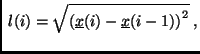
In conjunction with eqn (2), the length of each sail element has to be kept constant.
Along with the boundary condition of fixed
sail ends, a corrected force can be determined as a constant to start with eqn (1) again.
This iterative process is continued until a certain level of convergence is reached.
due to the flow solution on each element,
eqns (1) and (2) are considered. Eqn (1) gives an
explicit expression for the nodal forces that can be calculated depending on the
force on the first node which can be arbitrarily initialized.
In conjunction with eqn (2), the length of each sail element has to be kept constant.
Along with the boundary condition of fixed
sail ends, a corrected force can be determined as a constant to start with eqn (1) again.
This iterative process is continued until a certain level of convergence is reached.
Afterwards, displacements resulting from the change in sail shape are imposed on the grid and a new grid is computed, and the computation can be proceeded by one time step again.
3 Results
The fully coupled computations are started at ![]() angle of attack where the
sail shape is awaited to be stable and separation bubbles should be small - if existent at all.
After convergence,
the angle is raised step by step up to a chosen maximum of
angle of attack where the
sail shape is awaited to be stable and separation bubbles should be small - if existent at all.
After convergence,
the angle is raised step by step up to a chosen maximum of ![]() far beyond separation, and
on another ``computational branch'' decreased step by step to an angle, where the
algorithm fails to give a solution, fig. 2. In this case the incidence angle has become negative below
a critical value, where tension in the sail is close to zero and luffing occurs.
Lowering the angle further, a hysteresis would occur. Thus, the sail shape
becomes unstable and the deformations exceed the validity of the method, which cannot yet handle luffing
that occurs earlier at higher excess lengths. However, the algorithm gives stable
solutions for negative incidence close to
far beyond separation, and
on another ``computational branch'' decreased step by step to an angle, where the
algorithm fails to give a solution, fig. 2. In this case the incidence angle has become negative below
a critical value, where tension in the sail is close to zero and luffing occurs.
Lowering the angle further, a hysteresis would occur. Thus, the sail shape
becomes unstable and the deformations exceed the validity of the method, which cannot yet handle luffing
that occurs earlier at higher excess lengths. However, the algorithm gives stable
solutions for negative incidence close to ![]() .
The onset of numerical divergence roughly matches the angle where luffing occurs in the experiments.
.
The onset of numerical divergence roughly matches the angle where luffing occurs in the experiments.
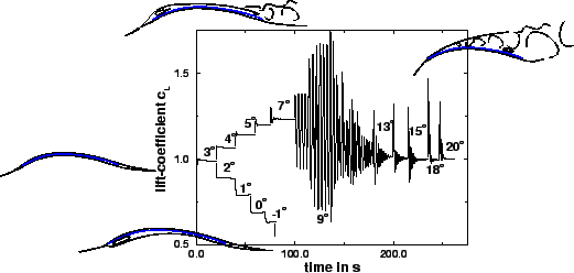
| Figure 2: | Evolution of lift coefficient vs. time for varying angle of attack during computation and schematic drawings of streamlines around sail at different angles. |
Computational results are presented as diagrams of lift coefficient vs. angle
of attack for three different excess lengths, in fig. 3
for
![]() (left) and
(left) and
![]() (right), and in fig. 4
for
(right), and in fig. 4
for
![]() (left), for a Reynolds number based on chord length of
(left), for a Reynolds number based on chord length of
![]() obtained on grids with 16.000 control volumes covering a physical domain
of
obtained on grids with 16.000 control volumes covering a physical domain
of
![]() from
from ![]() to
to ![]() and
and
![]() from
from ![]() to
to ![]() at
at
![]() and
and ![]() to
to ![]() at
at
![]() , fig. 1.
This number was found sufficient when evaluating the effects of grid refinement on the prediction of lift
for these excess lengths. As low-Reynolds-number boundary conditions were used, the wall-normal distance
, fig. 1.
This number was found sufficient when evaluating the effects of grid refinement on the prediction of lift
for these excess lengths. As low-Reynolds-number boundary conditions were used, the wall-normal distance ![]() of the first grid points was kept around
of the first grid points was kept around ![]() .
The computations are compared to experimental results and a linear approximation
.
The computations are compared to experimental results and a linear approximation
| (7) |
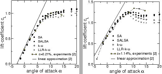
| Figure 3: | Lift coefficient versus angle of attack for excess length
|
At low angles of attack good agreement can be found with the linear approximation as well as with
the experimental results for small excess lengths.
For
![]() , the shortest sail, no distinctive maximum in computed lift can be seen,
whereas for longer sails the loss in lift after separation increases and a maximum
lift coefficient originates roughly at
, the shortest sail, no distinctive maximum in computed lift can be seen,
whereas for longer sails the loss in lift after separation increases and a maximum
lift coefficient originates roughly at ![]() , its height dependent on the sail length.
For
, its height dependent on the sail length.
For
![]() there are only very few experimental data points, so comparability
is very poor, moreover, only the one-equation models obtained stable solutions. In this
case the loss in lift due to separation is significantly underpredicted and the linear
approximation does not hold anymore at all, either.
there are only very few experimental data points, so comparability
is very poor, moreover, only the one-equation models obtained stable solutions. In this
case the loss in lift due to separation is significantly underpredicted and the linear
approximation does not hold anymore at all, either.
This reveals that approaching onset of separation, the computational results depend strongly on subtle details pertaining to the representation of turbulence. The one-equation models capture most of the experimental results but fail to render the effects of massive separation, whereas the other models tend to produce more separation resulting in a lower lift coefficient at lower angle of attack. Grid-refinement posed even more problems with stability in these cases, revealing that the effects of inertia and damping on the sail shape computation will have to be studied.
The results for lift with separation are averaged values as the flow becomes unsteady before full
separation has developed.
Fig. 1 shows the extremely unsteady behaviour of the system at these incidence angles for
![]() .
Unfortunately, this behaviour is not represented in any experimental result, so nothing
can be said about the physical reliability of the frequency computed, which is roughly
.
Unfortunately, this behaviour is not represented in any experimental result, so nothing
can be said about the physical reliability of the frequency computed, which is roughly ![]() Hz,
which corresponds to a Strouhal number
Hz,
which corresponds to a Strouhal number
![]() of lower than 0.03 in this case. At least, turbulent
and mean flow frequencies can thus be estimated to be around three orders of magnitude apart, Rung [9],
so that applying RANS methods to these unsteady flows does not contradict the basic assumptions of
statistical turbulence modelling.
of lower than 0.03 in this case. At least, turbulent
and mean flow frequencies can thus be estimated to be around three orders of magnitude apart, Rung [9],
so that applying RANS methods to these unsteady flows does not contradict the basic assumptions of
statistical turbulence modelling.
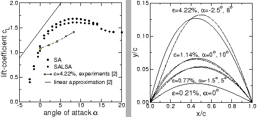
| Figure 4: | Lift coefficient versus angle of attack for excess length
|
With higher excess length
![]() not
only the maximum lift but also the sail deformation grows, fig. 4 (right), and the
grid-deformation algorithm has to meet these requirements. This can easily be
done with the proposed procedure as long as the sail deformation is small.
When luffing occurs and the sail snaps through, the loss in grid quality is to
high for the procedure to work.
not
only the maximum lift but also the sail deformation grows, fig. 4 (right), and the
grid-deformation algorithm has to meet these requirements. This can easily be
done with the proposed procedure as long as the sail deformation is small.
When luffing occurs and the sail snaps through, the loss in grid quality is to
high for the procedure to work.
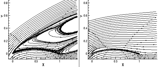
| Figure 5: | Streamlines for LLR- |
In figs. 5 and 6 streamline pictures are shown for angles of attack ![]() ranging from
ranging from ![]() to
to
![]() .
For high angles of attack beyond maximum lift, fig. 5 (left), the flow is fully separated
on the upper side of the sail and steady vortices occur in the wake with a similar streamline pattern
and pressure distribution for angles of attack above
.
For high angles of attack beyond maximum lift, fig. 5 (left), the flow is fully separated
on the upper side of the sail and steady vortices occur in the wake with a similar streamline pattern
and pressure distribution for angles of attack above ![]() .
.
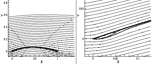
| Figure 6: | Streamlines for LLR- |
For lower angles of attack, fig. 5 (right), the streamlines reveal a separation bubble limited in size
on the upper side that is also visible in the ![]() distribution. This separation bubble
grows with increasing angle of attack until it becomes unstable in size.
Due to the sharp leading edge - the sail has zero thickness - this separation only vanishes when
streamlines and sail are nearly parallel at the front, fig. 6 (left), roughly at
distribution. This separation bubble
grows with increasing angle of attack until it becomes unstable in size.
Due to the sharp leading edge - the sail has zero thickness - this separation only vanishes when
streamlines and sail are nearly parallel at the front, fig. 6 (left), roughly at ![]() .
.
On the other hand, when the angle of attack decreases, a separation bubble occurs on the lower side of the sail, fig. 6 (right), only visible in a magnification or the pressure distribution. In this case the sail is more and more likely to become unstable or snap through.
4 Conclusions and Outlook
The chain model works in conjunction with the RANS-method and
all turbulence models investigated are able to capture the experimental results at low angle of
attack and
the weakly non-linear area is predicted with success for small excess lengths
![]() .
In case of massive separation and for long sails, however, severe deviations and differences between the turbulence models show up
and between the experiments and computations.
.
In case of massive separation and for long sails, however, severe deviations and differences between the turbulence models show up
and between the experiments and computations.
Hence, more research is considered necessary and additional effects will have to be taken into account,
such as transitional effects and three-dimensionality.
Moreover, work in progress is directed towards
higher-order closure models and obtaining and evaluating more experimental data.
Another step will be the introduction of
damping and inertia into the sail algorithm to stabilize the procedure which will be necessary
for the computation of a full hysteresis including luffing and to be able to handle even higher
excess lengths
![]() .
An examination of the effects of grid refinement on the frequency of oscillations and sail shape is
also considered necessary.
.
An examination of the effects of grid refinement on the frequency of oscillations and sail shape is
also considered necessary.
To further validate the procedure against analytical results for
small excess lengths
![]() , inviscid computations are aimed at,
together with laminar computations as a starting point for introducing fixed and variable transition
in a next step. So far, inviscid computations could not be performed due to the loss in
stability of the numerical procedure when viscosity is small.
, inviscid computations are aimed at,
together with laminar computations as a starting point for introducing fixed and variable transition
in a next step. So far, inviscid computations could not be performed due to the loss in
stability of the numerical procedure when viscosity is small.
Acknowledgment
This research was partly funded by the Deutsche
Forschungsgemeinschaft (DFG-SFB 557 'Beeinflussung komplexer turbulenter Scherströmungen').
References