In order to simplify the existing EASM and to achieve an efficient numerical implementation the underlying tensor basis plays an important role. The five-term tensor basis that is introduced here tries to combine an optimum of accuracy of the complete basis with the advantages of a pure 2d concept. Therefor a suitable five-term basis is identified. Based on that the new model is designed and validated in combination with different eddy-viscosity type background models.

In the frame work of single-point closures (Reynolds-stress transport models = RSTM) still provide the best representation of flow physics. Due to numeric requirements an explicit formulation based on a low number of tensors is desirable and was already introduced [6] [5]. Originally most explicit algebraic stress models are formulated using a 10-term basis:

The reduction of the tensor basis however requires an enormous mathematical effort. Rung [3] guided a way to transform the algebraic stress formulation for a given linear algebraic RSTM into a given tensor basis by keeping all important properties of the underlying model. This transformation can be applied to an arbitrary tensor basis. In the present investigations an optimum set of basis tensors and the corresponding coefficients is to be found.

The projection method was introduced by Jongen et al [2] to enable an approximate solution of the algebraic transport equation of the Reynolds-stresses. In contrast to the approach of Gatski et al [1], the tensor basis is not inserted in the algebraic equation, instead the algebraic equation is projected. Therefore, the chosen basis tensors does not need to form a complete integrity basis. However, the projection will fail if the basis tensor are linear dependent. In the case of a complete basis the projection leads to the same solution as the direct insertion, otherwise an approximate solution in the sense of an least squares method is obtained.

In order to prove, that the projection method will lead to the same solution as the direct insertion, the EASM for two-dimensional flows is derived. In two-dimensional flows only the tensors

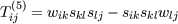
are independent. As shown in [3] the projection leads then to the same coefficients as the approach of Gatski et al [1]. This two-dimensional EASM is used as starting point for an optimized EASM which includes three-dimensional effects. For example the shear stress variation in a rotating pipe can not be predicted with quadratic tensors. Hence, the EASM was extended with a cubic tensor. In order to do not affect the performance in two-dimensional flows, a tensor was chosen that vanish in 2d flows. This offers the concentration of the coefficient determination in 3d flows. A cubic tensor, which vanishes in 3d flow is:

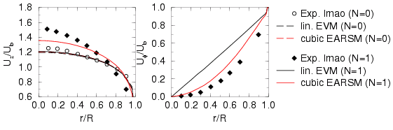
The projection with tensors T⁽¹⁾, T⁽²⁾, T⁽³⁾ and T⁽⁵⁾ yields then the coefficients of the EASM. The performance of the derived cubic EASM is depicted in Figure 1. Due the rotation the shear stress is reduced and the axial velocity increased. At the rotation rate  = 0 a steady pipe flow is obtained. In this case both model predict the same flow. However, when the pipe rotates (N=1), the linear eddy-viscosity model shows a linear circumferential velocity, which corresponds to a solid body rotation. In contrast the cubic EASM leads to a parabolic profile like in the experiment.

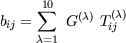
Figure 1: Axial and circumferential velocities in an axial rotating pipe at rotation rates (N=0) and (N=1) compared to Experiments by Imao .

With regard to an improved prediction of normal stress anisotropy in 3d flows the EASM was extended with a quartic tensor. Like the cubic tensor the quartic tensor should vanish in 2d flow situations. Therefore, the quartic tensor was combined with a quadratic tensor and reads:

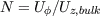
At the present different simplifications of the resulting projection matrix are investigated to obtain an optimized coefficient set.

limitation of

A direct result of the EASM derivation is a variable formulation of . As the generators of the extended EASM where chosen to preserve the existing 2D formulation the expression of remains unchanged:

A_i are the constants of the underlying pressure-strain model.

Since is always positive it might be possible that becomes singular. Therefore in the first EASM derivation of Gatski et al. [1] a regularization was introduced, which prevent a singular by cutting the range of . However, Wallin et al. pointed out that the regularization detoriated the performance of the EASM. In their model the methodology was refined to account for the coefficient

This leads to a weak non-linear conditional equation for the EASM coefficients and an additional equation for g must be solved. In 3D the equation of g is of 6th order, wherefore a closed solution is only possible in 2D flows, where the equation reduces to 3rd order. In order to circumvent the root finding of a polynomial equation Rung [3] established a quasi-selfconsistent approach. He showed that by using a expression of a realizable linear model instead of the EASM- expression in the equation of g the same properties of g follows. For a wide range of and the quasi-selfconsistent approach is almost identical to the fully selfconsistent solution of Wallin. Thus the quality of the EASM is not affected with the advantage of no additional non-linear equation.

The extension of the 2D-EASM by two 3D generators introduced in the preceding paragraph do not change the coefficient g. The traces of the new generators multiplied by s (i.e. T⁵_ijs_ij and T⁸"_ijs_ij) identically vanish. However, it should be noted that the 2D part itself leads to a different expression for as the invariant arises. But since in the projections to determine the EASM coefficients the complexity is reduced by neglecting higher order invariants.

1. Gatski, T.B. and Speziale, C.G., "On explicit algebraic stress models for complex turbulent flows". J. Fluid Mech., 254, pp. 59-78, 1993
2. Jongen, T. and Gatski, T.B., "General explicit algebraic stress relations and best approximations for three-dimensional flows", Int. J. Engineering Science, 36, pp. 739, 1998
3. Rung, T., "Entwicklung anisotroper Wirbelzähigkeitsbeziehungen mit Hilfe von Projektionstechniken", PHD-thesis, Technical University Berlin, 2000
4. Rung, T., Lübcke, H., Franke, M., Thiele, F. and Fu, S., "Assessment of Explicit Algebraic Stress Models in Transonic Flows", Eng. Turbulence Modelling and Experiments 4, pp. 659-668, 1999.
5. Taulbee, D.B., "An improved algebraic Reynolds stress model and corresponding nonlinaer stress model", Phys. Fluids, 28, pp 2555-2561, 1992.
6. Wallin, S. and Johansson, A.V., "A new explicit algebraic Reynolds stress turbulence model including an improved near-wall treatment", Flow Modelling and Turbulence Measurements IV, A.A. Balkema, pp. 309-406, 1996.
7. Fu, S., Qian, W. and Zhang, G., Development of Nonlinear Eddy-viscosity Model for Numerical Simulation of Three-Dimensional turbulent Boundary Layer, Eng. Turbulence Modelling and Experiments 5, Mallorca, 2002.
8. Lübcke, H.; Rung, T.; Thiele, F. "Prediction of the Spreading Mechanism of 3D Turbulent Wall Jets with Explicit Reynolds-Stress Closures", Eng. Turbulence Modelling and Experiments 5, Mallorca, 2002.